mm-ADT is a dual licensed AGPL3/commercial open source project that offers software engineers, computer scientists, mathematicians, and others in the software industry a royalty-based OSS model. The Turing Complete mm-ADT virtual machine (VM) integrates disparate data technologies via algebraic composition, yielding synthetic data systems that have the requisite computational power and expressivity for the problems they were designed to solve. As an economic model, each integration point offers the respective development team access to the revenue streams generated by any for-profit organization leveraging mm-ADT.
Virtual Machine Components
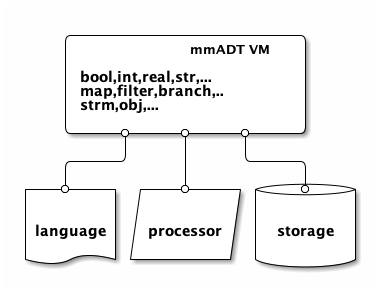
The mm-ADT VM integrates the following data processing technologies:
-
Programming Languages: Language designers can create custom languages or develop parsers for existing languages that compile to mm-ADT VM assembly code (
mmlang) or bytecode (binary encoding ofmmlang). -
Processing Engines: Processor developers can enable their push- or pull-based execution engines to be programmed by any mm-ADT language. The abstract processing model supports single-machine, multi-threaded, agent-based, distributed near-time, and/or cluster-oriented, batch-analytic processors.
-
Storage Systems: Storage engineers can expose their systems via model-ADTs expressed in mm-ADT’s dependent type system that enable the lossless encoding of key/value store, document store, wide-column store, graph store, relational store, and other novel or hybrid structures such as hypergraph, docu-graph, and quantum data structures.
The mm-ADT VM enables the intermingling of any language, any processor, and any storage system that can faithfully implement the core language semantics (types and values), processor semantics (instruction set architecture), and/or storage semantics (data structure streams).
mm-ADT Theory
mm-ADT Function
Every mm-ADT program denotes a single unary function that maps an obj of type \$S\$ (start) to an obj of type \$E\$ (end) with the function signature
\[ f: S \rightarrow E. \]
The complexities of mm-ADT are realized in the definition of an obj (which includes both types and values) and the internal structure of an \$f\$-program (which is a composition of nested curried functions). The sole purpose of this documentation is to make salient the various algebraic structures that are operationalized to ultimately yield the mapping \$f : S \rightarrow E\$.
mm-ADT Algebras

The base algebra of mm-ADT is a type-oriented ring algebra called the obj stream ring. There are three surjective homomorphisms from the obj stream ring to the algebras of the aforementioned components. The language algebra's free monoid enables the nested, serial composition of parameterized instructions (inst) from the mm-ADT instruction set architecture and is called the inst monoid. The processor algebra is called the type ringoid and it is a free polynomial ringoid (poly) at compilation and non-free ringoid at evaluation. The storage algebra is called the obj monoid and it maintains a carrier set composed of all mm-ADT objects (obj) and an associative, binary operator for constructing data streams.
These component algebras represent the particular perspective that each component has on a shared data structure called the obj graph. This graph has a faithful encoding as a generalized Cayley graph and a commutative diagram. It serves as the medium by which the virtual machine’s computations take place: from specification, to compilation and then evaluation.
| Component | Algebra |
|---|---|
language |
|
processor |
|
storage |
|
The primary purpose of this documentation is to explain these algebras, specify their relationship to one another and demonstrate how they are manipulated by mm-ADT technologies. Data system engineers will learn how to integrate their technology so end users may compose their efforts with others' to create synthetic data systems tailored to a problem’s particular computational requirements.
mm-ADT Technology
mm-ADT Console
The mm-ADT VM provides a REPL console for users to evaluate mm-ADT programs written in any mm-ADT language.
The reference language distributed with the VM is called mmlang. mmlang is a low-level, functional language that is in near 1-to-1 correspondence with the underlying VM architecture — offering it’s users Turing-Complete expressivity when writing programs and an interactive teaching tool for studying the mm-ADT VM.
~/mm-adt bin/mmadt.sh
                                _____ _______
                           /\  |  __ |__   __|
 _ __ ___  _ __ ___ _____ /  \ | |  | | | |
| '_ ` _ \| '_ ` _ |_____/ /\ \| |  | | | |
| | | | | | | | | | |   / ____ \ |__| | | |
|_| |_| |_|_| |_| |_|  /_/    \_\____/  |_|
                                 mm-adt.org
mmlang>
A simple console session is presented below, where the parser expects programs written in the language specified left of the > prompt.
All the examples contained herein are presented using mmlang.
mmlang> 1
==>1
mmlang> 1+2
==>3
mmlang> 1[plus,2]
==>3
mmlang Syntax and Semantics
The context-free grammar for mmlang is presented below. Every mmlang expression denotes an element of the free inst monoid.
obj   ::= (type | value)q
value ::= vbool | vint | vreal | vstr
vbool ::= 'true' | 'false'
vint  ::= [1-9][0-9]*
vreal ::= [0-9]+'.'[0-9]*
vstr  ::= "'" [a-zA-Z]* "'"
type  ::= ctype | dtype
ctype ::= 'bool' | 'int'  | 'real' | 'str' | poly | '_'
poly  ::= lst | rec | inst
q     ::= '{' int (',' int)? '}'
dtype ::= ctype q? ('<=' ctype q?)? inst*
sep   ::= ';' | ',' | '|'
lst   ::= '(' obj (sep obj)* ')' q?
rec   ::= '(' obj '->' obj (sep obj '->' obj)* ')' q?
inst  ::= '[' op(','obj)* ']' q?
op    ::= 'a' | 'add' | 'and' | 'as' | 'combine' | 'count' | 'eq' | 'error' |
          'explain' | 'fold' | 'from' | 'get' | 'given' | 'groupCount' | 'gt' |
          'gte' | 'head' | 'id' | 'is' | 'last' | 'lt' | 'lte' | 'map' | 'merge' |
          'mult' | 'neg' | 'noop' | 'one' | 'or' | 'path' | 'plus' | 'pow' | 'put' |
          'q' | 'repeat' |'split' | 'start' | 'tail' | 'to' | 'trace' | 'type' | 'zero'
The Type
Category theory is the study of structure via morphisms that expose (or generate) other structures. Two important category theoretic concepts dealing with substructures are products and coproducts.

A product is any object defined in terms of it’s accessible component objects. That is, from a single object, via \$\pi_n\$ projection morphisms, the product is decomposed into it’s constituent parts.

A coproduct is any object defined in terms of the component objects used to construct it. That is, from many objects, via \$\iota_n\$ injection morphisms, a coproduct can be composed from constituent parts.
Along with these decomposition (and composition) morphisms, there exists an isomorphism between any two products (or coproducts) should they project (or inject) to the same component objects. That is, product and coproduct equality are defined via component equality.
Types and Values
Everything that can be denoted in mmlang is an obj.
Within the VM and outside the referential purview of an interfacing language, every obj is the product of

-
an object that is either a type object or a value object and
-
a quantifier specifying the "amount" of objects being denoted.
\[ \begin{split} \text{ } \\ \texttt{obj} &= \texttt{object} &\;\times\; \texttt{q} \text{ } \\ \texttt{obj} &= (\texttt{type object} + \texttt{value object}) &\;\times\; \texttt{q}. \end{split} \]

This internal structure is well-defined as an algebraic ring.
The ring axioms specify how the internals of an obj are related via two binary operators: \$\times\$ and \$\+\$ . One particular axiom states that products both left and right distribute over coproducts.
Thus, the previous formula is equivalent to
\[ \texttt{obj} = (\texttt{type object} \times \texttt{q}) + (\texttt{value object} \times \texttt{q}). \]
There are two distinct kinds of mm-ADT objs: quantified type objects and quantified value objects. These products of the obj coproduct are called by simpler names: type and value.
That is the obj meta-model.
\[ \texttt{obj} = \texttt{type} + \texttt{value} \]
There are only a few instances in which it is necessary to consider the object component of an obj separate from its quantifier component.
The terms type and value will always refer to the object/quantifier-pair as a whole — i.e., an obj.
|
mmlang> int              (1)
==>int
mmlang> 1                (2)
==>1
mmlang> int{5}           (3)
==>int{5}
mmlang> 1{5}             (4)
==>1{5}
mmlang> ['a','b','a']    (5)
==>'b'
==>'a'{2}| 1 | A single int type. |
| 2 | A single int value of 1. |
| 3 | Five int types. |
| 4 | Five 1 int values. |
| 5 | A str stream composed of 'a','b', and 'a' (definition forthcoming). |
Both types and values can be operated on by types, where each is predominately the focus of either compilation (types) or evaluation (values).
-
\$ (\tt{type} \times \tt{type}) \rightarrow \tt{type} \$: Used in compilation for type inferencing and type rewriting, and
-
\$ (\tt{value} \times \tt{type}) \rightarrow \tt{value} \$: Used in program evaluation and as lambda functions.
mmlang> int => int[is,[gt,0]]                   (1)
==>int{?}<=int[is,bool<=int[gt,0]]
mmlang> 5 => int{?}<=int[is,bool<=int[gt,0]]    (2)
==>5| 1 | Compilation: The int-type is applied to the int[is,[gt,0]]-type to yield a maybe int{?}-type. |
| 2 | Evaluation: The nested bool<=int[gt,0]-type is a lamba function yielding true or false. |
Some interesting conceptual blurs arise from the intermixing of types and values. The particulars of the ideas in the table below will be discussed over the course of the documentation.
| structure A | structure B | unification |
|---|---|---|
type |
program |
a program is a "complicated" type. |
compilation |
evaluation |
compilations are type evaluations, where a compilation error is a "type runtime" error. |
type |
variable |
types refer to values across contexts and variables refer to values within a context. |
type |
a single intermediate representation is used in compilation, optimization, and evaluation. |
|
type |
function |
functions are (dependent) types with values generated at evaluation. |
state |
trace |
types and values both encode state information in their process traces. |
classical |
quantum |
quantum computing is classical computing with a unitary matrix quantifier ring. |
Type Structure

A Cayley graph is a graphical encoding of a group. If \$(A, \cdot, I)\$ is a group with carrier set \$A\$, binary operator \$\cdot : (A \times A) \to A\$, and generating set \$I \subseteq A\$ then the graph \$G = (V,E)\$ with vertices \$V = A\$ and labeled edges \$E = A \times I \times A\$ is the Cayley graph of the group. The directed edge \$(a,i,b) \in E\$ written \$a \to_i b\$ states that the vertices \$a,b \in A\$ are connected by an edge labeled with the element \$i \in I\$. Thus, \$a \to_i b\$ captures the group operation \$a \cdot i = b\$.
When constructed in full, a Cayley graph’s vertices are the group elements and its edges represent the set of all possible \$I\$-transitions between elements. When lazily constructed, a Cayley graph encodes the history of a group computation, where the current element has an incoming \$I\$-edge from the previous element. A Cayley graph captures both the proto-free and non-free aspects of a group. The non-free aspect is realized by any edge \$e = (a,i,b)\$ such that \$ai \mapsto b\$ and an element of the corresponding free algebra \$(A^\ast,\ast)\$ can be constructed by concatenating the edge labels of a path \$\prod_{e \in (a,i,b)^\ast} \pi_1(e)\$.
A generalized Cayley graph does not require that every \$i \in I\$ have a corresponding \$i^{-1} \in I\$ such that \$i \cdot i^{-1} = \mathbf{1}\$ (i.e., multiplicative inverses). By lifting this constraint, the Cayley graphical structure can be used to encode other magmas such as monoids and semigroups.
An obj is either a type or a value:
\[
\texttt{obj} = \texttt{type} + \texttt{value}.
\]
That equation is not an axiom, but a theorem.
Its truth can be deduced from the equations of the full axiomatization of obj.
In particular, for types, they are defined relative to other types.
Types are a coproduct of either a
-
canonical type (ctype): a base/fundamental type, or a
-
derived type (dtype): a product of a type and an instruction (
inst).
The ctypes are nominal types. There are five ctypes:
-
bool: denotes the set of booleans — \$ \mathbb{B} \$.
-
int: denotes the set of integers — \$ \mathbb{Z} \$.
-
real: denotes the set of reals — \$ \mathbb{R} \$.
-
str: denotes the set of character strings — \$ \Sigma^\ast \$.
-
poly: denotes the set of free objects — \$ \tt{obj}^\ast \$.

The dtypes are structural types whose recursive definition's base case is a ctype realized via a chain of instructions (inst) that operate on types to yield types. In other words, instructions are the generating set of a type monoid. Formally, the type coproduct is defined as
\[ \begin{split} \texttt{type} &=\;& (\texttt{bool} + \texttt{int} + \texttt{real} + \texttt{str} + \texttt{poly}) + (\texttt{type} \times \texttt{inst}) \\ \texttt{type} &=\;& \texttt{ctype} + (\texttt{type} \times \texttt{inst}) \\ \texttt{type} &=\;& \texttt{ctype} + \texttt{dtype}. \end{split} \]
Every obj has an associated quantifier.
When the typographical representation of an obj lacks an associated quantifier, the quantifier is unity.
For instance, the real 1.35{1} is written more economically as 1.35.
|
A dtype has two product projections. The type projection denotes the domain and the instruction projection denotes the function, where the type product as a whole, relative to the aforementioned component projections, is the range. \[ \begin{split} \tt{type} &=\;& (\tt{type} &\;\times\;& \tt{inst}) &\;+\;& \tt{ctype} \\ \text{“range} &=\;& (\text{domain} &\;\text{and}\;& \text{function}) &\;\text{or}\;& \text{base"} \end{split} \]
The implication of the dtype product is that mm-ADT types are generated inductively by applying instructions from the mm-ADT VM’s instruction set architecture (inst). The application of an inst to a type (ctype or dtype) yields a dtype that is a structural expansion of the previous type.

For example, int is a ctype. When int is applied to the instruction [is>0], the dtype int{?}<=int[is>0] is formed, where [is>0] is syntactic sugar for [is,[gt,0]]. This dtype is a refinement type that restricts int to only those int values greater than zero — i.e., a natural number \$\mathbb{N}^+\$.
In terms of the "range = domain and function" reading, when an int (domain) is applied to [is>0] (function), the result is either an int greater than zero or no int at all {?} (range).

The diagram above captures a fundamental structure in mm-ADT called the obj graph. The obj graph is used for, amongst other things, type checking, type inference, compiler optimization, and garbage collection. The subgraph concerned with type definitions is called the type graph. The subgraph encoding values and their relations as a function of the types is called the value graph. The obj graph is also the codomain of an embedding whose domain is an obj ringoid called the stream ring. Both the obj graph and stream ring form the primary topics of study in this documentation.
The obj meta-model structure thus far is diagrammed on the right (with quantifiers attached to each component). On the left are some example mmlang expressions.

mmlang> int                                                         (1)
==>int
mmlang> int{2}                                                      (2)
==>int{2}
mmlang> int{2}[is>0]                                                (3)
==>int{0,2}<=int{2}[is,bool{2}<=int{2}[gt,0]]
mmlang> int{2}[is>0][plus,[neg]]                                    (4)
==>int{0,2}<=int{2}[is,bool{2}<=int{2}[gt,0]][plus,int{0,2}[neg]]
mmlang> 5{2} => int{2}[is>0][plus,[neg]]                            (5)
==>0{2}| 1 | A ctype denoting a single integer. |
| 2 | A ctype denoting two integers. |
| 3 | A dtype denoting zero, one, or two integers greater than 0. |
| 4 | A dtype extending the previous type with negative integer addition. |
| 5 | A value of two fives applied to the previous type with the result being two 0s. |
Type Components
The illustration below highlights the two primary components of a type, where an edge of the Cayley graph is the triple \$e=(a,i,b) \in (\tt{type} \times \tt{i\nst} \times \tt{type})\$.
-
Type signature: the ctype specification of a type’s domain and range.
-
Type definition: a domain rooted instruction sequence terminating at the range.

| An image referred to as a diagram or commuting diagram is isomorphic to the system of equations it captures and thus, respects the axioms of the algebraic structure being diagrammed. An image referred to as an illustration is intended to elicit a realization of the associated topic via intuition and should not be considered a faithful encoding of an underlying mathematics. |
Type Signature
Every mm-ADT type can be generally understood as a function that maps an obj of one type to an obj of another type. A type signature specifies the source and target of this mapping, where the domain is the source type, and the range is the target type. In mmlang a type signature has the following general form where {q} is the ctype’s associated quantifier.
|
| In common mathematical vernacular, if the function \$f\$ has a domain of \$X\$ and a range (codomain) of \$Y\$, then its signature is denoted \$f: X \to Y\$. Furthermore, with quantifiers in \$Q\$, the function signature would be denoted \$f: X \times Q \to Y \times Q\$ or \$f: (X \times Q) \to (Y \times Q)\$. |
| mmlang Expression | Description |
|---|---|
|
From the perspective of "type-as-function," An mm-ADT |
|
In most programming languages, a value can be typed
Such declarations state that the value referred to by |
|
|
|
Quantifiers must be elements from a ring with unity. In the previous examples, the quantifier ring was \$(\mathbb{Z}, +,\ast)\$. In this example, the quantifier ring is \$(\mathbb{Z} \times \mathbb{Z}, +,\ast)\$, where the carrier set is the set of all pairs of integers and addition and multiplication operate pairwise,
\[
(a,b) \ast (c,d) \mapsto (a \ast c,b \ast d).
\]
The type |
|
Types that are fully specified by their type signature are canonical types (ctypes). Therefore, |
Type Definition
Category theory is a branch of abstract algebra that studies, among other things, arbitrary algebraic structures via their homomorphic embedding in a multi-sorted monoid called a category. A category \$\mathcal{C}\$ is denoted \[ (\mathbf{C} ,\circ ,\mathbf{1}), \] where \$\mathbf{C}\$ is a set-family of morphisms, \$\circ: \mathbf{C} \times \mathbf{C} \rightarrow \mathbf{C}\$ is an associative binary morphism composition operator, and for every identity morphism \$\mathbf{1}_A \in \mathbf{1}\$, \$\mathbf{1}_A \circ \mathbf{1}_A = \mathbf{1}_A\$ denotes an object that is more simply written \$A\$ such that \$A \mapsto \mathbf{1}_A\$. The family set \$mathbf{C}\$ indexes hom-sets with \$\mathbf{C}(A,B)\$ denoting all morphism between objects \$A\$ and \$B\$, where \$f:A\to B \in \mathbf{C}(A,B)\$ and \$id: A \rightarrow A \cong \mathbf{1}_A \cong A\$.
Unlike classical monoids, a category’s \$\circ\$ operator is generally not closed. That is, there are compositions which may not be defined. It is this aspect of a category that makes it a multi-sorted (or typed) monoid.

The discipline of category theory makes extensive use of a homomorphism from a category to a directed labeled graph called a diagram. These diagrams realize the same underlying unitary operation of the generators of a magma within a generalized Cayley graph. If \$f:A \to B\$ and \$g: B \to C\$, then there exists the morphism path \[ A \xrightarrow{f} B \xrightarrow{g} C, \] which, in Cayley graph notation, is denoted \$A \to_f B \to_g C\$. An important subset of diagrams are the commutative diagrams. In a commutative diagram every morphism path starting at the same source and ending at the same destination are considered equivalent (with respects to equivalence in the respective algebraic structure being modeled categorically). Thus, if \$g \circ f = i \circ h\$, then it is said that the above diagram commutes.
Types and values both have a ground that exists outside of the mm-ADT virtual machine within the hosting environment (e.g. the JVM). The ground of the mm-ADT value 2 is the JVM primitive 2L (a Java long). The ground of the mm-ADT type int is the JVM class java.lang.Long. When the instruction [plus,4] is applied to the mm-ADT int value 2, a new mm-ADT int value is created whose ground is the JVM value 6L. When [plus,4] is applied to the mm-ADT int type, a new type is created with the same java.lang.Long ground. Thus, the information that distinguishes int from int[plus,4] is in the reference to the instruction that was applied to int.
 For a type, the deterministic chain of references is called the type definition and is encoded as a path in the type graph. For a value, the value graph encodes a path called the value history. The commutative diagram below is composed of two horizontal paths. The top path is a value history and the bottom path is a type definition. These paths are joined by the
 [type] instruction which are diagrammed using hook-tailed arrows that denote, by convention, a monomorphic embedding known more simply as an inclusion (i.e., \$a \in A\$ or \$A' \subset A\$). The set of all [type] morphisms is equivalent to the hom-set \$\tt{Hom}(\tt{value},\tt{type})\$ which defines a functor that specifies a particular embedding of the value graph into the type graph. This aggregate structure is of import in mm-ADT. It’s called the obj graph.
In theory, the complete history of an mm-ADT program (from compilation to execution) is stored in the obj graph. However, in practice, the mm-ADT VM removes paths once they are no longer required by the program.
This process is called path retraction and is the mm-ADT equivalent of garbage collection.
|
|

| In practice, the string representation of a value is its ground and the string representation of a type is its path. |
 To provide a preview of what is to come, an mm-ADT model defines an
 obj graph for a particular domain of discourse. A transition from model \$A\$ to model \$B\$ may be possible by way of a functor derived from \$\tt{Hom}(A,B)\$. Furthermore, it may be possible to go from \$A\$ to \$\tt{mm}\$ via a composition with \$\tt{Hom}(B,\tt{mm})\$. Two such parallel compositions between models are illustrated in the associated diagram and written as
\[
\begin{split}
\texttt{Hom}(A,B) &\circ \texttt{Hom}(B,\texttt{mm}) \\
\texttt{Hom}(A,C) &\circ \texttt{Hom}(C,\texttt{mm}).
\end{split}
\]
Model mappings allow types written in one universe to be evaluated within another universe, where, ultimately, all types must be grounded in the base mm model. The specification and selection of paths to mm is determined by mm-ADT programs that leverage model libraries. Ultimately, it is through mm that the mm-ADT VM communicates with storage systems and processing engines, enabling arbitrary models atop a sound evaluation.
The obj graph is both a generalized Cayley graph of a partial monoid and the commutative diagram (or quiver) of the category composed of obj vertices and inst labeled edges. More generally, the obj graph is the graph of unary functions comprising inst, where instructions operate on both types and values.
From compilation to evaluation, depending on the particular context, either interpretation will be leveraged.
-
Commutative diagram: vertices denote type/value-objects of the
objcategory withinstmorphisms.
The obj graph’s commuting property eases compile-time and runtime type rewriting.
If two paths have the same source vertex (domain) and target vertex (range), then both paths yield the same result (the target vertex).
In practice, evaluating the instructions along the computationally cheaper path is prudent.

-
Cayley graph: vertices denote type/value-elements of the
instmonoid with generating edges ininst.
As a generalized, multi-rooted monoidal Cayley graph, the set of all possible mm-ADT computations is theoretically predetermined given the monoid presentation containing the root objs (e.g. the ctypes), its generators (inst), and relations (path equations).
This static immutable structure serves to memoize computational results.
This is especially useful when considering streams (definition forthcoming) and their role in data-intensive, cluster-oriented environments where storage is cheap and processors are costly.
Type Quantification
A category may have an initial and/or terminal object.

An initial object \$S\$ is the domain of a set of morphism \$S \rightarrow E_n\$. Initial objects, via their morphisms, generate all the objects of the category. If there is an initial object, then it is unique in that if there is another initial object, it has the same diagrammatic topology — all outgoing morphisms and no incoming morphisms save the identity. Thus, besides labels, two initials are isomorphic.

A terminal object \$E\$ is the range of a set of morphisms \$S_n \rightarrow E\$. Terminal objects subsume all other objects in the category in that all other objects \$S_n\$ can be morphed into the terminal object, but the terminal object can not be morphed into any other object. Similar to initials, should another terminal exist, the two terminal are isomorphic in that they both have the same number of incoming morphisms and no outgoing morphisms (save the identity).
In order to quantify the amount of values denoted by a type, every mm-ADT type has an associated quantifier \$q \in Q\$ written {q} in mmlang, where \$Q\$ is the carrier of an ordered algebraic ring with unity (e.g. integers \$\mathbb{Z}\$, reals in \$ \mathbb{R}, \mathbb{R}^2, \mathbb{R}^3, \ldots, \mathbb{R}^n \$, unitary matrices, etc.).
|
Typically, integer quantifiers signify "amount." However, other quantifiers such as unitary matrices used in the representation of a quantum wave function, "amount" is a less accurate description as objs interact with constructive and destructive interference. Even in \$\mathbb{Z}\$, negative integers are possible and are leveraged for computing lazy set operations as demonstrated by intersection in the associated example.
The default quantifier ring of the mm-ADT VM is
\[
(\mathbb{Z} \times \mathbb{Z}, +, \ast),
\]
where \$(0,0)\$ is the additive identity and \$(1,1)\$ is the multiplicative identity (unity). The \$ +\$ and \$\ast\$ binary operators perform pairwise integer addition and multiplication, respectively. In mmlang if an obj quantifier is not displayed, then the quantifier is assumed to be the unity of the ring, or {1,1} in this case. Moreover, if a single value is provided, it is assumed to be repeated, where {n} is shorthand for {n,n}. Thus,
|
\[ \texttt{int} \equiv \texttt{int{1}} \equiv \texttt{int\{1,1\}}. \]
One particular quantifier of every ring serves an important role in mm-ADT as both the additive identity and multiplicative annihilator — {0}.
All objs quantified with the respective quantifier ring’s annihilator are non-terminal initial objects as exemplified in the adjoining example.
Types such as |
Quantifiers serve an important role in type inference and determining, at compile time, the expected cost of a particular type definition (i.e., an instruction sequence). The table below itemizes common quantifier patterns that have a corresponding construction in other programming languages.
| name | sugar | unsugared | description | mmlang example |
|---|---|---|---|---|
some |
|
a single |
|
|
option |
|
|
0 or 1 |
|
none |
|
|
0 |
|
exact |
|
|
4 |
|
any |
|
|
0 or more |
|
given |
|
|
1 or more |
|
Types use quantifiers in two separate, but related, contexts: type signatures and type definitions.
Type Signature Quantification
A type signature’s domain specifies the type and quantity of the obj required for evaluation. The range denotes what can be expected in return. int{6}<=int{3} states that given 3 ints, the type will return 6 ints.
Quantifiers in a type signature are descriptive, used in type checking.
mmlang> 4 => int{6}<=int{3}[[plus,1],[plus,1]]
language error: int is not an int{3}
mmlang> 4{3} => int{6}<=int{3}[[plus,1],[plus,1]]
==>5{6}
mmlang> [4,5,6] => int{6}<=int{3}[[plus,1],[plus,1]]
==>5{2}
==>6{2}
==>7{2}
mmlang> [4{2},5{1},6{2}] => int{6}<=int{3}[[plus,1],[plus,1]]
language error: int{5} is not an int{3}
mmlang> [4{2},5{-1},6{2}] => int{6}<=int{3}[[plus,1],[plus,1]]
==>5{4}
==>6{-2}
==>7{4}
Much will be said about negative quantifiers. For now, note that negative quantifiers enable lazy, stream-based set theoretic operations such as intersection, union, difference, etc. Extending beyond integer quantification \$(\mathbb{Z})\$, negative quantifiers enable constructive and destructive interference in quantum computating \$(\mathbb{C})\$ and excitatory and inhibitory activations in neural computing \$(\mathbb{R})\$.
Type Definition Quantification
A type definition’s instructions can be quantified. More specifically, a type’s intermediate dtypes can be quantified. During type inference, the quantifier ring’s \$(+\$/\$\ast)\$-operators propagate the quantifiers through the types that compose the program.
mmlang> int{3}[[plus,1],[plus,1]]              (1)
==>int{6}<=int{3}[plus,1]{2}
mmlang> int{3}[plus,1]{2}                      (2)
==>int{6}<=int{3}[plus,1]{2}| 1 | Given 3 ints, [plus,1] will be evaluated (in parallel) twice. The result is 6 ints. |
| 2 | The instruction [plus,1]{2} is the merging of two [plus,1] branches. |
At type compilation, the branch optimizer "collapses" type object equivalent branches with no effect to the result. The branches' type quantifiers are added using the quantifier ring’s \$+\$-operator (the quantifier group). Once collapsed, quantifiers can be moved left-or-right using the quantifier ring’s multiplicative \$\ast\$-operator due to the commutativity of quantifiers theorem (the quantifier monoid). It is more efficient (especially as branches grow in complexity) to compute, for example, \$2b\$ than \$b + b\$. The example below demonstrates how type quantifiers are "collapsed" with \$ +\$ and "slid" left (or right) with \$\ast\$.
\[ \begin{split} a(b+b)c &= a(2b)c \\ &= a2bc \\ &= 2abc \end{split} \] |
|

The following two examples highlight the fact that type signature quantifiers are used for type checking and type definition quantifiers are used for type inference. The algebra of quantification will be explained in much more detail later when discussing the ring algebra of mm-ADT.
|
\[ \begin{split} \texttt{int{q}} &= 3 \ast (1 + 1) \\ &= (3 \ast 1) + (3 \ast 1) \\ &= 3 + 3 \\ &= 6 \end{split} \] |
|
\[ \begin{split} \texttt{int{q}} &= 3 \ast 2 \\ &= 6 \end{split} \] |
Quantifier Commutativity
Each of these expressions is equivalent to |
|
All three expression evaluate to the same |
|
If the quantifier ring is not commutative, it is still possible to propagate coefficients left or right through an |
|
Quantifiers propagate along the the multiplicative |
|
Type Composition

Stream ring theory studies a particular type of algebraic ring constructed from a direct product of a function semiring and coefficient ring. Along with the standard ring axioms over \$\ast\$ and \$ \+\$, the theory requires that every stream ring uphold five additional axioms regarding coefficient dynamics. Categorically, every stream ring forms an additive category with biproducts. A biproduct has both projection (product) and injection (coproduct) morphisms that capture the splitting and merging of streams. Along with the atemporal stream theorem derived from the stream ring axioms, biproduct streams have practical significance in asynchronous distributed computing environments that primarily enjoy embarrassingly parallel processing, but where, at certain space and time synchronization points, data needs to be co-located by the reduce near-ring operator \$\oplus\$.
mm-ADT adopts the algebra of stream ring theory, but uses the term instruction for function and quantifier for coefficient. Moreover, mm-ADT extends stream ring theory with an inductive, dependent type theory based on a multi-sorted stream ring with interval quantifiers called the type ringoid whose free algebra is captured by the type graph.
\[ \big[ m_0 \ast m_1 \ast \ldots \ast m_n \big] \begin{bmatrix} g_0 \\ + \\ g_1 \\ + \\ \vdots \\ + \\ g_n \end{bmatrix} \left| \oplus r \right\rangle \big[ \ast \ldots \ast \big] \begin{bmatrix} + \\ \vdots \\ + \\ \end{bmatrix} \ldots \] |
The mm-ADT virtual machine has two distinct algebraic layers: the instruction set architecture and the stream ring. The instructions (inst) specify how input objs are mapped to output objs and has a graphical realization as a generalized Cayley graph and/or a commuting diagram. The inst algebra is evaluated by the processor-oriented stream ring algebra. A stream ring has three operators for constructing types: \$\ast\$, \$ +\$, and \$\oplus\$, where the first two are the classic ring operators and the last is particular to a stream ring. The stream ring’s multiplicative monoid’s \$\ast\$-operator concatenates serial streams, the additive abelian group’s \$ +\$-operator composes parallel streams, and the stream near-ring’s non-commutative group’s \$\oplus\$-operator reduces streams down to a singleton stream.
| op | inst | sugar |
|---|---|---|
\$\ast\$ |
|
|
\$ +\$ |
|
|
\$ \oplus\$ |
|
|
The illustration above is an intuitive visualization of an mm-ADT type from the perspective of monoidal, group, and near-ring magmas interacting with one another in a series (\$\ast\$) of expansions (\$ +\$) and contractions (\$ \oplus\$), where \$m_i,g_i,r \in \tt{obj}\$. These three stream operators have a corresponding realization in inst as higher-order instructions. It is through these instructions that the other instructions are grounded in the underlying stream ring algebra of the mm-ADT VM.
Stream Ring Operators
An obj is defined
\[
\texttt{obj} = (\texttt{type} \times \texttt{q}) + (\texttt{value} \times \texttt{q}).
\]
Thus, an obj is either a quantified type or a quantifier value. With respects to the stream ring’s three operators, there are 4 binary obj configurations (\$2^2\$) that each operator will encounter: value/value, value/type, type/value, and type/type. The table below presents the equations of each operator for each of the 4 configurations, where it is through operations involving right-hand side (RHS) types that the instructions in inst are applied to objs (e.g., \$t(v)\$ is evaluation and \$t(t)\$ is compilation). Thus, the stream ring is the fundamental algebra of the mm-ADT VM.
In the examples to follow, a term of the form \$x_q\$ is a type (\$t\$) or value (\$v\$) with quantifier \$q\$ and \$\mathbf{x}\$ is a stream of types or values, where an \$i \in \mathbb{N}\$ as in \$\mathbf{x}_i\$ denotes the \$i^{\text{th}}\$ obj of \$\mathbf{x}\$.
|
| \$\cdot\$ | [juxt] => |
[branch] =[ |
[barrier] =| |
|---|---|---|---|
value \$\cdot\$ value |
\[ {v_0}_{q} \Rightarrow {v_1}_{r} = {v_1}_{q \ast r} \] |
\[ [{v_0}_{q},{v_1}_{r}] = \begin{cases} {v_0}_{q + r} & \text{if } v_0 == v_1 \\ [{v_0}_q,{v_1}_r] & \text{otherwise}. \end{cases} \] |
\[ \mathbf{v} ⫤ {v_1}_r = {v_1}_r \] |
value \$\cdot\$ type |
\[ v_q \Rightarrow t_r = t(v)_{q \ast r} \] |
\[ [v_q,t_r] = [v_q,t_r] \] |
\[ \mathbf{v} ⫤ t_r = \left(\bigoplus_{i=0}^n t(\mathbf{v}_i)\right)_r \] |
type \$\cdot\$ value |
\[ t_q \Rightarrow v_r = v_{q \ast r} \] |
\[ [t_q,v_r] = [t_q,v_r] \] |
\[ \mathbf{t} ⫤ v_r = v_r \] |
type \$\cdot\$ type |
\[ {t_0}_q \Rightarrow {t_1}_r = t_1(t_0)_{q \ast r} \] |
\[ [{t_0}_{q},{t_1}_{r}] = \begin{cases} {t_0}_{q + r} & \text{if } t_0 == t_1 \\ [{t_0}_q,{t_1}_r] & \text{otherwise}. \end{cases} \] |
\[ \mathbf{t_0} ⫤ t_1 = \left(\bigoplus_{i=0}^n t_1(\mathbf{t_0}_i)\right)_r \] |
The simple example program below uses all 3 stream ring operators. The subsequent table provides a detailed decomposition of the evaluation. The instruction [model,mmx] loads the mm-ADT extension model that contains common mm base type coercions such as int<=str, real<=int, etc.
mmlang> :[model,mmx]
==>_
mmlang> 4 => int[mult,2] => str[plus,'0'] => real
==>80.0
mmlang> 4 => int[mult,2] =[ int=>str[plus,'0'],int=>str[plus,'.1'] ] => real
==>80.0
==>8.1
type |
|
|
|
|
|---|---|---|---|---|
d/r |
|
|
|
|
value |
|
|
|
|
q |
|
|
|
|
op |
\$ast\$ monoid |
\$+\$ abelian group |
\$\ast\$ monoid |
\$\oplus\$ group |
term |
series |
expansion |
series |
contraction |
Stream Ring Algebra
The mm-ADT stream ring is the algebraic ring \[ (\texttt{obj},+,\ast,\oplus,\mathbf{0},\mathbf{1}), \]
where

-
\$\tt{obj}\$ is the carrier set containing all quantified objects,
-
\$+\$ the additive parallel branch operator,
-
\$\ast\$ the multiplicative serial chain operator,
-
\$\oplus\$ is the reducing barrier operator,
-
\$\mathbf{0}\$ the additive identity, and
-
\$\mathbf{1}\$ the multiplicative identity.
The equation \$\tt{obj} = \tt{type} + \tt{value}\$) and the suggestive illustration above highlight two important uses of the ring’s multiplicative binary \$\ast\$-operator:
-
\$\ast: \tt{type} \times \tt{type} \to \tt{type}\$ generate functions graph (program compilation) and,
-
\$\ast: \tt{value} \times \tt{type} \to \tt{value}\$ stream values through the type structure (program evaluation).
Along with the standard ring axioms (save operator closure), the obj stream ring respects the five additional axioms of stream ring theory.
The following tables provide a consolidated summary of the ring axioms, stream ring axioms and their realization in mm-ADT via examples in mmlang using both obj values and types.
The mmlang examples are rife with syntactic sugars.
The term _{0} (sugar’d {0}) is \$\mathbf{0}\$, _{1} (sugar’d {1}) is \$\mathbf{1}\$, [a,b,c] denotes [branch,(a,b,c)] and +{q}n denotes [plus,n]{q}.
Finally, while [,] and [;] are defined as binary operators, due to the associativity axioms of the respective additive group and multiplicative monoid of a ring, [,] and [;] are effectively \$n\$-ary operators and will be used as such in examples to follow.
|
Ring Axioms
Axioms are the "hardcoded" equations of a system. Regardless of any other behaviors the system may express, if the system always respects the ring axioms, then the system is (in part) a ring.
| axiom | equation | mmlang values | mmlang types |
|---|---|---|---|
Additive Abelian Group — \$(\tt{obj},+,\mathbf{0})\$ |
|||
Additive associativity |
\[\begin{split} &(a+b)+c \\ =& a+(b+c) \end{split}\] |
|
|
Additive commutativity |
\[\begin{split} &a+b \\ =& b+a \end{split}\] |
|
|
Additive identity |
\[a+\mathbf{0} = a\] |
|
|
Additive inverse |
\[a + ({-a}) = \mathbf{0}\] |
|
|
Multiplicative Monoid — \$(\tt{obj},\ast,\mathbf{1})\$ |
|||
Multiplicative associativity |
\[\begin{split} &(a \cdot b) \cdot c \\ =& a \cdot (b \cdot c) \end{split}\] |
|
|
Multiplicative identity |
\[a \cdot \mathbf{1} = a\] |
|
|
Ring with Unity — \$(\tt{obj},+,\ast,\mathbf{0},\mathbf{1})\$ |
|||
Left distributivity |
\[\begin{split} &a \cdot (b + c) \\ =& ab + ac \end{split}\] |
|
|
Right distributivity |
\[\begin{split} &(a+b) \cdot c \\ =& ac + bc \end{split}\] |
|
|
Ring Theorems
The axioms of a theory entail its theorems. Stated in reverse, theorems are the derivations of an axiomatic system. Once a system is determined to be a ring, then all the theorems that have been proved about rings in general are also true for that system.
| theorem | equation | mmlang values | mmlang types |
|---|---|---|---|
Ring with Unity — \$(\tt{obj},+,\ast,\mathbf{0},\mathbf{1})\$ |
|||
Additive factoring |
\[\begin{split} &a + b = a + c \\ ⇒& b = c \end{split}\] |
||
Unique factoring |
\[\begin{split} &a + b = \mathbf{0} \\ ⇒& a = -b \\ ⇒& b = -a \end{split}\] |
||
Inverse distributivity |
\[\begin{split} &-(a+b) \\ =& (-a) + (-b) \end{split}\] |
|
|
Inverse distributivity |
\[-(-a) = a\] |
|
|
Annihilator |
\[\begin{split} &a*\mathbf{0} \\ =& \mathbf{0} \\ =& \mathbf{0}*a \end{split}\] |
|
|
Factoring |
\[\begin{split} &a * (-b) \\ =& -a * b \\ =& -(a*b) \end{split}\] |
|
|
Factoring |
\[\begin{split} &(-a) * (-b) \\ =& a * b \end{split}\] |
|
|
Stream Ring Axioms

Stream ring theory studies quantified objects. The quantifiers must be elements of an ordered ring with unity. The stream ring axioms are primarily concerned with quantifier equations and their relationship to efficient stream computing. The most common quantifier ring is integer pairs (denoting a range) with standard pairwise addition and multiplication, \$(\mathbb{Z} \times \mathbb{Z},+,\ast,(0,0),(1,1))\$. However, the theory holds as long as the quantifiers respect the ring axioms and, when coupled to an object, they respect the stream ring axioms.
The algebra underlying most type theories operate as a semiring(oid), where the additive component is a monoid as opposed to an invertible group.
In mm-ADT, the elements of the additive component can be inverted by their corresponding negative type (or negative obj in general).
Thus, mm-ADT realizes an additive groupoid, where, for example, the ,-poly [int{1},int{-1}] is int{0} which is isomorphic to the initial obj{0}.
|
| axiom | equation | mmlang values | mmlang types |
|---|---|---|---|
Bulking |
\[\begin{split} & xa + ya \\ =& (x+y)a \end{split}\] |
|
|
Applying |
\$xa \ast yb = (xy)ab\$ |
|
|
Splitting |
\[\begin{split} & xa \ast (yb + zc) \\ =& (xy)ab + (xz)ac \end{split}\] |
|
|
Merging |
\[\begin{split} & ((xa) + (yb)) \\ =& (xa + yb) \end{split}\] |
|
|
Removing |
\[ (\mathbf{0}a + b) = b \] |
|
|
Type System
mm-ADT’s type system is founded on 3 classes of ctypes: anonymous, mono, and poly types. Within the mono and poly types, further subdivisions exist. These foundational types are the building blocks by which all other types are constructed using the ring operators of mm-ADT’s stream ring algebra. At the limit, an mm-ADT program is best understood as a "complex" type.
Anonymous Types
The type bool<=int[gt,10] has a range of bool and a domain of int. When the type is written without it’s range as int[gt,10], the range is deduced. The int domain ctype is applied to [gt,10] to yield a bool. A type with an unspecified range is called an an anonymous type and is denoted _ in mmlang (or with no character in many situations). An anonymous range is the result of an anonymous domain.
_ range |
_ domain |
||||||||||||||
|---|---|---|---|---|---|---|---|---|---|---|---|---|---|---|---|
|
|
In the anonymous type |
|
|
|

Anonymous Type Uses
Anonymous types are useful in other situations besides lazy typing expressions.
mmlang> 5-<(_,_)                               (1)
==>(5{2})
mmlang> -5[is>0 -> +2 | _ -> +10]              (2)
==>5
mmlang> 5-<([a,int],[a,_],[a,str])             (3)
==>(true{2},false)| 1 | When no processing is needed on a split, _ should be provided. |
| 2 | When used in a |-rec poly, _ is used to denote the default case. |
| 3 | 5 is both an int and a _, but not a str. |
In general, anonymous types are wildcards because they pattern match to every obj. As will be demonstrated soon, when a variable is specified (e.g. [plus,x]) or a new type is specified (e.g. x:42), The x is a named anonymous type. The entailment of this is that types and variables are in the same namespace. Two presumably self-explanatory examples are provided below with a more detailed discussion of variables and named types forthcoming.
| variables | named types |
|---|---|
|
|
Mono Types
| type | inst | 0 | 1 |
|---|---|---|---|
|
|
|
|
|
|
|
|
|
|
|
1.0 |
|
|
|
The mm-ADT type system can be partitioned into mono types (monomials) and poly types (polynomials). There are 4 mono types, each denoting a classical primtive data type: bool, int, real, and str. The associated table presents the typical operators (sugared instructions) that can be applied to each mono type. The table also includes their respective additive \$(\mathbf{0})\$ and multiplicative \$(\mathbf{1})\$ identities.
A few of the more interesting aspects of the mono types are detailed in the following subsections.
Zero and One
The instructions [zero] and [one] are constant polymorphic instructions. Each provides a unique singleton value associated with the type of the respective incoming obj. In the example to follow, = is sugar for pairwise [combine], with round robin evaluation for overflow. As examples, (a,b,c)=(x,y) yields (ax,by,cx) and (a,b,c)=(x) is (ax,bx,cx) (i.e.,right scalar multiplication).
mmlang> (true;6;5.5;'ryan')=([zero])
==>(false;0;0.0;'')
mmlang> (true;6;5.5)=([one])
==>(true;1;1.0)
mmlang> 'ryan'[one]
language error: 'ryan' is not supported by [one]
Each type’s \$\mathbf{0}\$ and \$\mathbf{1}\$ value serves as the [plus] and [mult] instruction identities, respectively. Furthermore, for types respecting a ring with unity algebra, [zero] is their corresponding multiplicative annihilator.
mmlang> (true;6;5.5;'ryan')=(+[zero])
==>(true;6;5.5;'ryan')
mmlang> (true;6;5.5)=(*[one])
==>(true;6;5.5)
mmlang> (true;6;5.5)=(*[zero])
==>(false;0;0.0)
Poly Types
A poly is a free object. Free objects are universal structures in that they respect the equations of an abstract algebra, but not the equations of an instance of the abstract algebra. Hence the term free as in "free" from constraint of the concrete—i.e., universal. Examples of these two classes of equations are provided in the table below. If the concrete algebra equations appear random, it is because they are. Each concrete algebra’s operator(s) map elements-to-elements in a manner specific to an application domain and as such, are not universal equations.
| abstract algebra equations | concrete algebra equations | |
|---|---|---|
\$a \cdot \mathbf{1} = a\$ |
\$a \cdot b = b\$ |
|
\$a \cdot a^{-1} = \mathbf{1}\$ |
\$a \cdot b^{-1} = \mathbf{1} \$ |
|
\$a \cdot (b \cdot c) = (a \cdot b) \cdot c\$ |
\$(a \cdot b) \cdot c = b \cdot c\$ |
|
\$a \cdot b = b \cdot a\$ |
\$a \cdot a = a\$ |
In mm-ADT, polys are
-
collection data structures, where the collection’s semantics are tied to the operator(s) of the free object’s abstract algebra, and
-
control data processes, where the control semantics are likewise a consequence of the underlying free object’s algebra.
The mm-ADT poly is versatile because it is agnostic to the types and values contained therein while remaining in one-to-one correspondence with the stream ring algebra's operators' axioms and entailed theorems. More poetically, poly is the bedrock upon which the mm-ADT algebraic ecology is sustained.
Poly Types and Values
There are type polys and there are value polys. A type poly contains at least one type obj and is typically intended for use as a flow control structure. A value poly is composed of only value objs with a common use as a collection data structure.
As a practical consideration, mm-ADT offers two kinds of poly: lst (list) and rec (record), where theoretically, rec is simply a lst with some added conveniences that make typical programming patterns easier to express. Finally, a poly is associated with one of three algebras that comprise mm-ADT’s stream ring: , (abelian group), ; (monoid), or | (near-ring).
\[ \begin{split} \texttt{poly} &= \texttt{lst} &+ \texttt{rec} \\ \texttt{poly} &= (\texttt{,-lst} + \texttt{|-lst} + \texttt{;-lst}) &+ (\texttt{,-rec} + \texttt{|-rec} + \texttt{;-rec}). \end{split} \]

| poly | sep | access | value | type |
|---|---|---|---|---|
|
|
all |
||
|
last |
|||
|
head |
|||
|
|
all match |
||
|
last match |
|||
|
first match |
There are three instructions that are of primary importance for poly with one being a composite of the other two.
-
[split](-<): propagates an incomingobjthrough apolyaccording to its algebra. -
[merge](>-): aggregates outgoingobjsfrom apolyaccording to its algebra. -
[branch](=[): propagates and then aggregatesobjsthrough apolyaccording to its algebra.
The details of these instructions will be discussed in full over the following subsections.
| mmlang | mmnotation | |
|---|---|---|
|
\$\ast\$ |
\[\tiny{\prod}\] |
|
\$ +\$ |
\[\tiny{\coprod}\] |
|
\$\oplus\$ |
\[\tiny{\bigoplus}\] |
The mmlang notation is able to denote every possible type through the obj graph. That is, is can be used to define automata that can recognize every possible path through the obj graph. A companion notation exists separate from mmlang which is more aligned with the formalisms used in standard mathematical treatments of an algebraic system. This notation is called mm notation.
-
Monoidal composition (\$\ast\$): A non-branch serial path through the
objgraph is expressed with the multiplicative \$\Pi\$ operator. Given sequence of types \$\mathbf{a} = [a_0,a_1,\ldots,a_n]\$, their monoidal composition is denoted \[ \prod_{i=0}^{n} \mathbf{a}_i \;\;\;\;\text{ or }\;\;\;\; \mathbf{a}_\ast \] where, for the latter, it is implied that entire sequence is left-to-right composed (via fold) using the stream ring multiplicative \$\ast\$-operator. While the first representation is more verbose, it’s use will become apparent when considering intermediate operations within a monoidal composition. -
Groupoidal composition (\$+\$): Parallel paths through the
objgraph is denoted with the respective additive operator. Thus, given \$n\$-independent types \$\mathbf{a} = [a_0,a_1,\ldots,a_n]\$, their parallel evaluation is denoted \[ \coprod_{i=0}^n \mathbf{a}_i \;\;\;\;\text{ or }\;\;\;\; \mathbf{a}_{ +} \] -
Near-ring reduction (\$\oplus\$): A path barrier is denoted with the \$\oplus\$ reduction operator. Given \$n\$-types (serial or parallel), their reduction using using the function \$f:A^{\ast} \to B\$ is denoted \[ \bigoplus_{i=0}^n f(\mathbf{a}_i) \;\;\;\;\text{ or }\;\;\;\; \mathbf{a}_{\oplus f} \]
It is important to note that the composition operator on the vector representation is portrayed bottom right. The reason being is that regular language syntax is reserved for the top right. Next, in order to apply the same \$m\$-serial types to \$n\$-parallel types the additive and multiplicative operators are used in conjunction. \[ \begin{split} \coprod_{i=0}^n \mathbf{a}_i \prod_{j=0}^m \mathbf{b}_j &= (\mathbf{a}\mathbf{b}_{*})_{ +} \\ &= (a_0\mathbf{b}_{\ast} + a_1\mathbf{b}_{\ast} + \ldots + a_n\mathbf{b}_{\ast}) \\ &= (a_0 b_0 b_1 \ldots b_m) + \ldots + (a_n b_0 b_1 \ldots b_m) \end{split} \] The additive/multiplicative pattern emphasizes the monoid ring interpretation of mm-ADT as well as the well know ring property that every ring is isomorphic to the composition of endomorphisms (\$ \ast \$) of the ring’s additive abelian group (\$ +\$), where each \$a_i\$ group element has applied a series of \$\mathbf{b}\$ morphisms back to the carrier set (i.e., an endomorphism).
Poly Collections
A poly can be used a collection data structure. There are a total of 6 sorts of collections as there are two kinds of poly (lst and rec) and each kind has 3 algebras (,,;,|).
| lst | collection | mmlang example | rec | collection | mmlang example |
|---|---|---|---|---|---|
|
|
|
|
||
|
|
|
|
||
|
|
|
|
,-poly Collections
The ,-polys capture the additive abelian group of the mm-ADT stream ring.
| abstract magma | stream magma | free poly |
|---|---|---|
\[(\tt{obj}, +, \mathbf{0})\] |
\[(\texttt{obj},\texttt{[branch]},\{\mathbf{0}\})\] |
\[(\texttt{obj},\texttt{(,)},\{\mathbf{0}\})\] |
A general ,-poly has obj as its carrier set, , as its the commutative binary \$+\$-operator, and {0} (_{0}) as its identity element. With obj quantification, should two ,-poly terms have equal objects, they can be merged according to the mm-ADT [branch] operator equation:
\[
[\texttt{branch},a_q, b_r] =
\begin{cases}
a_{q + r} & \text{if } a == b, \\
[\texttt{branch},a_q, b_r] & \text{otherwise},
\end{cases}
\]
where \$+\$ is the quantifier ring’s additive operator and
\[
[a_q,\{\mathbf{0}\}] = a_q.
\]
The commutative aspect of the ,-poly does not enforce an order upon its elements which yields set-like semantics. However, given quantifier "weighting," ,-lst collections realize multiset semantics (also known as bags or weighted sets) and ,-rec collections realize multimap semantics (associative arrays with multiple values for a single key).
A few self-explanatory ,-poly examples are provided below.
| ,-lst | ,-rec |
|---|---|
|
|
;-poly Collections
The ;-polys capture the non-commutative, multiplicative monoid of the mm-ADT ring.
| abstract magma | stream magma | free poly |
|---|---|---|
\[(\tt{obj}, \ast, \mathbf{1})\] |
\[(\texttt{obj},\texttt{[juxt]},\texttt{[noop]})\] |
\[(\texttt{obj},\texttt{(;)},\{\mathbf{1}\})\] |
The ;-poly carrier set is obj, the multiplicative operator is ;, the multiplicative identity is {1}, and due to the larger ring in which this magma is embedded, {0} is the annihilator. Due to non-commutativity, the ; delimited elements form an ordered sequence. In lst, the consequence is a collection data structure with list-semantics. In rec, a record with ordered fields is realized. Both support duplicates so the rec form is less like an associative array and more like a list of pairs/fields.
The [juxt] operator is mm-ADT’s multiplicative monoid operator and is only applied in ;-poly for the universal elements \$\mathbf{1}\$ and \$\mathbf{0}\$. Given the equation
\[ a_q[\texttt{juxt}, b_r] = \begin{cases} b_{q \ast r} & \text{if } b \text{ is a value}, \\ b(a)_{q \ast r} & \text{otherwise,} \end{cases} \\ \]
;-poly only computes the free monoid identity
\[
a_q\texttt{[juxt,[noop]]} = a_q.
\]
Examples are presented below that contain both \$\{\mathbf{0}\}\$ and \$\{\mathbf{1}\}\$ elements.
| ;-lst | ;-rec |
|---|---|
|
|
|-poly Collections
The |-polys captures endomorphic, left-distributive, multiplicative, compositions over the near-ring subgroup of mm-ADT’s additive abelian group.
| abstract magma | stream magma | free poly |
|---|---|---|
\[(\texttt{obj},\oplus_1,\mathbf{0}/\mathbf{1})\] |
\[(\texttt{obj},\texttt{[barrier,[head]]},\{\mathbf{1}\},\{\mathbf{0}\})\] |
\[(\texttt{obj},\texttt{(|)},\{\mathbf{1}\},\{\mathbf{0}\})\] |
The [barrier] \$n\$-ary operator’s arguments are all the objs of the input stream. This yields a blocking synchronization point necessary for reduce/fold-based computations. The operator’s \$1\$ subscript denotes a particular augmentation to the higher-order \$\oplus\$ operator, where \$\oplus_1\$ returns the first non-zero obj argument — i.e., the head of the stream (a lazy computation).
\[ \begin{split} [a_q,\ldots,b_r]\texttt{[barrier,[head]]} &= \begin{cases} a_q & \text{if } q > 0, \\ \ldots \\ b_r & \text{if } r > 0, \\ \{\mathbf{0}\} & \text{otherwise,} \end{cases} \end{split} \]
|-poly yields singleton lsts and recs. The purpose of this seemingly odd behavior is more salient in |-polys flow controls (presented in the next section). A collection of self-explanatory examples are provided below.
| |-lst | |-rec |
|---|---|
|
|
When each poly contains 0 or 1 element, the respective algebras behave equivalently. It is only at 2+ terms that the poly algebras become discernible and instructions such as [eq] consider the poly element separator in their calculation.
|
Poly Controls
The mm-ADT ring’s additive abelian group operator is accessible via the [branch] instruction. The [branch] instruction’s argument is a poly. Each term of the poly argument is an operand of the ring’s \$+\$-operator. In this way, each of the 6 poly forms represents a particular control structure. Due to the prevalent use of [branch], mmlang offers the sugar’d encoding of [ ], where both the instruction opcode and the poly parentheses are not written. For example, [branch,(+1,+2,+3)] is equivalent to [+1,+2,+3].
| lst | control | mmlang example | rec | control | mmlang example |
|---|---|---|---|---|---|
|
|
|
|
||
|
|
|
|
||
|
|
|
|
In the examples to follow, the elements of the polys are labeled by first letter of their algebraic structure: \$g\$ is abelian group, \$m\$ is monoid, and \$r\$ is near-ring. For the rec examples, the key elements are labeled with \$k\$. The mmlang examples use Unicode subscript characters and [plus] to compose \$x\$ with the objs along the respective data control path. These choices were purely aesthetic, driven by the desire to better align the examples with their respective illustrative diagrams and mm notation equations.
|
,-poly Controls
The ,-polys capture the additive abelian group of the mm-ADT stream ring. The associativity and commutativity of the group operator means that the order in which the terms are evaluated (associativity) and results aggregated (commutativity) does not change the semantics of the computation. More specifically to the notion of control, it means that the irreducible terms in a ,-poly are not sequentially dependent on one another. This independence enables evaluation isolation and thus, promotes parallelism. The ,-poly algebra realizes cascading union in lst and conditional cascading in rec.
| ,-lst (union cascade) | ,-rec (conditional cascade) |
|---|---|
\[ x ⇒ \big[g_0,g_1,\ldots,g_n\big] \;=\; \coprod_{i=0}^n x ⇒ g_i \] |
\[ x ⇒ \big[(k_0 \to g_0),\ldots,(k_n \to g_n)\big] \;=\; \coprod_{i=0}^n \begin{cases} x ⇒ g_i & \text{if } (x ⇒ k_i) \neq \mathbf{0}, \\ \mathbf{0} & \text{otherwise}. \end{cases} \] |
|
|
Branching can be understood as a two stage process which is captured by the [split]/[merge] instruction pairing. In practice, [split]/[merge] are useful in isolating a poly computation ([split]) to then later introduce the results ([merge]) into the outer stream. This is demonstrated below for ,-lst and ,-rec where -< is mmlang sugar for [split] and >- is mmlang sugar for [merge].
| ,-lst (union cascade) | ,-rec (conditional cascade) |
|---|---|
|
|
|
|


Note that in all subsequent [branch,poly] equations to follow, \$x \in \tt{obj}\$ is an incoming obj to the respective [branch] instruction.
;-poly Controls
The ;-polys capture the multiplicative monoid of the mm-ADT ring. The result of each term is the input to the next term in the sequence. In lst, method chaining is realized and in rec conditional chaining.
| ;-lst (fluent chaining) | ;-rec (conditional chaining) |
|---|---|
\[ x ⇒ \big[m_0;m_1;\ldots;m_n\big] \;=\; x ⇒ \prod_{i=0}^n m_i \] |
\[ x ⇒ \big[(k_0 \to m_0),\ldots,(k_n \to m_n)\big] \;=\; x ⇒ \prod_{i=0}^n \begin{cases} m_i & \text{if } (x ⇒ k_i) \neq \mathbf{0}, \\ \mathbf{0} & \text{otherwise}. \end{cases} \] |
|
|
 The
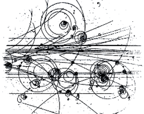
The ;-lst equation above realizes a structure and process joyfully named the "bubble chamber". In experimental higher-energy physics, a bubble chamber is small room filled with high pressure vapor. Particles are shot into the chamber and the trace they leave (called their varpor trail) provides physicists empirical data regarding the nature of the particle under study — e.g., its mass, velocity, spin, and, when capturing decay, the sub-atomic particles that compose it. As demonstrated below, \$x\$ is the particle and -< shoots \$x\$ into the ;-lst bubble chamber, where each term in the ;-lst acts as a vapor droplet.
| ;-lst (fluent chaining) | ;-rec (conditional chaining) |
|---|---|
|

|
|
|

|-poly Controls
The |-polys capture mm-ADT’s barrier near-ring, where the first non-\$\mathbf{0}\$ ("non-null") element is the output of the branch. As a control structure, |-poly is a sequential branch that can be understood programmatically as a short-circuit fold. In lst, non-null coalescing is realized and in rec a switch statement is realized.
| |-lst (coalesce) | |-rec (switch) |
|---|---|
\[ x ⇒ \big[r_0,r_1,\ldots,r_n\big] = \begin{cases} x ⇒ r_0 & \text{if } (x ⇒ r_0) \neq \mathbf{0}, \\ x ⇒ r_1 & \text{if } (x ⇒ r_1) \neq \mathbf{0}, \\ \ldots & \\ x ⇒ r_n & \text{if } (x ⇒ r_n) \neq \mathbf{0}, \\ \mathbf{0} & \text{otherwise}. \end{cases} \] |
\[ x ⇒ \big[(k_0\to r_0),\ldots,(k_n\to r_n)\big] = \begin{cases} x ⇒ r_0 & \text{if } (x ⇒ k_0) \neq \mathbf{0}, \\ x ⇒ r_1 & \text{if } (x ⇒ k_1) \neq \mathbf{0}, \\ \ldots & \\ x ⇒ r_n & \text{if } (x ⇒ k_n) \neq \mathbf{0}, \\ \mathbf{0} & \text{otherwise}. \end{cases} \] |
|
|
| |-lst (coalesce) | |-rec (switch) |
|---|---|
|
|
|
|


As previously stated for collection polys, control poly semantics are only discernible amongst polys with 2 or more terms.
|
Poly Lifting
 A consequence of the dual use of
 poly as both a data structure and a control structure is that poly supports a lifted encoding of mm-ADT itself. Each poly form captures a particular magma of the underlying mm-ADT stream ring algebra. As a collection, poly provides a programmatic way of writing mm-ADT programs (types) and as flow control, these poly encoded mm-ADT programs can be executed. The complete algebraic specification of poly lifting via an obj-module of the mm-ADT ring will be presented in a latter section. For now, the following mmlang examples demonstrate poly lifting in support of mm-ADT metaprogramming.
The mm-ADT type below contains both monoidal (serial composition) and group (parallel branching) components whose construction is captured by the bottom morphism of the diagram above. Note that the [explain] instruction is appended for educational purposes only — so as to detail the \$\Rightarrow\$ compositions.

mmlang> int{3}[mult,10][is>20 -> [+70,+170,+270],
                        is>10 ->   [*10,*20,*30]][plus,100][explain]
==>'
int{0,18}<=int{3}[mult,10][int{0,3}<=int{3}[is,bool{3}<=int{3}[gt,20]]->int{9}<=int{3}[int{3}[plus,70],int{3}[plus,170],int{3}[plus,270]],int{0,3}<=int{3}[is,bool{3}<=int{3}[gt,10]]->int{9}<=int{3}[int{3}[mult,10],int{3}[mult,20],int{3}[mult,30]]][plus,100]

inst                                           domain            range       state
-----------------------------------------------------------------------------------
[mult,10]                                      int{3}       =>   int{3}
[int{0,3}<=int{3}[is,bool{3}<=int{3}[gt,...    int{3}       =>   int{0,18}
 [is,bool{3}<=int{3}[gt,20]]                    int{3}      =>    int{0,3}
  [gt,20]                                        int{3}     =>     bool{3}
 ->[int{3}[plus,70],int{3}[plus,170],int{3}...    int{3}      =>    int{9}
  [plus,70]                                      int{3}     =>     int{3}
  [plus,170]                                     int{3}     =>     int{3}
  [plus,270]                                     int{3}     =>     int{3}
 [is,bool{3}<=int{3}[gt,10]]                    int{3}      =>    int{0,3}
  [gt,10]                                        int{3}     =>     bool{3}
 ->[int{3}[mult,10],int{3}[mult,20],int{3}[...    int{3}      =>    int{9}
  [mult,10]                                      int{3}     =>     int{3}
  [mult,20]                                      int{3}     =>     int{3}
  [mult,30]                                      int{3}     =>     int{3}
[plus,100]                                     int{0,18}    =>   int{0,18}
'
The above type can be expressed in a pure poly form, where ; is serial composition and , is parallel branching. This construction is captured by the slanted morphism in the diagram above.

mmlang> (int{3};[mult,10];-<(-<([is>20];-<(+70,+170,+270)>-)>-,
                             -<([is>10];-<(*10,*20,*30  )>-)>-)>-;[plus,100])
==>(int{3};_[mult,10];_[split,(_[split,(_[is,_[gt,20]];_[split,(_[plus,70],_[plus,170],_[plus,270])][merge])][merge],_[split,(_[is,_[gt,10]];_[split,(_[mult,10],_[mult,20],_[mult,30])][merge])][merge])][merge];_[plus,100])
The [split] instruction (sugar’d -<) renders poly a ring module. Incoming objs are scalars to a poly vector according to the equations
\[
\begin{split}
x \prec &\; (v_0,v_1,\ldots,v_n) \;\;&=\;\; (xv_0,xv_1,\ldots,xv_n) \\
x \prec &\; (v_0;v_1;\ldots;v_n) \;\;&=\;\; (xv_0;v_1;\ldots;v_n) \\
x \prec &\; (v_0|v_1|\ldots|v_n) \;\;&=\;\; (xv_i),
\end{split}
\]
where \$x \prec \tt{poly}\$ is the instruction x => [split,poly]. The [merge] instruction evaluates the poly according to the algebra denoted by its term separator (,, ;, or |). This has the effect of "draining" the poly of it’s internal objs such that
\[
\begin{split}
(xv_0,xv_1,\ldots,xv_n) \succ \;\;&=\;\; \coprod_{i=0}^n x \Rightarrow v_i \\
(xv_0;v_1;\ldots;v_n) \succ \;\;&=\;\; x \Rightarrow \prod_{i=0}^n v_i \\
(xv_i) \succ \;\;&=\;\; xv_i : v_i \neq \mathbf{0},
\end{split}
\]
where \$\tt{poly} \succ\$ is the expression poly => [merge].
Finally, both the original unlifted form and the poly lifted form of the type yield the same result at evaluation, where the final expression binds (-<) the values 1, 2, and 3 to the indeterminate terms, thus solving (>-) the polynomial equation.

mmlang> [1,2,3] => int{3}[mult,10][is>20 -> [+70,+170,+270],
                                   is>10 ->   [*10,*20,*30]][plus,100]
==>500
==>200
==>300{2}
==>400{2}
==>700{2}
==>1000
mmlang> [1,2,3]-<(int{3};[mult,10];-<(-<([is>20];-<(+70,+170,+270)>-)>-,
                                      -<([is>10];-<(*10,*20,*30  )>-)>-)>-;[plus,100])>-
==>500
==>200
==>300{2}
==>400{2}
==>700{2}
==>1000
Given that [split,poly:x][merge] is equivalent to [branch,poly:x], the poly type can be written more succinctly in a pure [branch] form as below.
mmlang> [1,2,3] => [int{3};[mult,10];[[[is>20];[+70,+170,+270]],
                                      [[is>10];[*10,*20,*30  ]]];[plus,100]]
==>500
==>200
==>300{2}
==>400{2}
==>700{2}
==>1000
Note that, when incident to each other, [split]/[merge] has the same equation as [branch].
\[ \begin{split} x \prec &\; (v_0,v_1,\ldots,v_n) \succ \;\;&=\;\; x \Rightarrow \big[v_0,v_1,\ldots,v_n \big] \;\;&=\;\; \coprod_{i=0}^n x \Rightarrow v_i \\ x \prec &\; (v_0;v_1;\ldots;v_n) \succ \;\;&=\;\; x \Rightarrow \big[v_0;v_1;\ldots;v_n\big] \;\;&=\;\; x \Rightarrow \prod_{i=0}^n v_i \\ x \prec &\; (v_0|v_1|\ldots|v_n) \succ \;\;&=\;\; x \Rightarrow \big[v_0|v_1|\ldots|v_n\big] \;\;&=\;\; xv_i : v_i \neq \mathbf{0} \end{split} \]
The reason for using -<( )>- versus [ ] is that when [split] and [merge] are not juxtaposed, reflection is possible on the intermediate results of the internal poly computation. That is, when only a [split] is applied, a half-branch occurs and all the poly domain instructions can operate on the midway results. Intuitively, [split] transforms a control structure into a data structure and [merge] transforms a data structure into a control structure. At this intermediate point when the computation is a data structure, the computation can be manipulated programmatically. That is the power of a lifted representation.
mmlang> [1,2,3]-<(int{3};[mult,10];-<(-<([is>20];-<(+70,+170,+270))))
==>(1;10;(({0};{0})))
==>(2;20;(({0};{0})))
==>(3;30;((30;(100,200,300))))
mmlang> [1,2,3]-<(int{3};[mult,10];-<(-<([is>20];-<(+70,+170,+270)),
                                      -<([is>10];-<(*10,*20,*30  ))))
==>(1;10;(({0};{0}),({0};{0})))
==>(2;20;(({0};{0}),(20;(200,400,600))))
==>(3;30;((30;(100,200,300)),(30;(300,600,900))))
mmlang> [1,2,3]-<(int{3};[mult,10];-<(-<([is>20];-<(+70,+170,+270)>-)>-,
                                      -<([is>10];-<(*10,*20,*30  )>-)>-)>-;[plus,100])
==>(1;10;{0};{0})
==>(2;20;[200,400,600];[300,500,700])
==>(3;30;[100,200,300{2},600,900];[200,300,400{2},700,1000])
mmlang> [1,2,3]-<(int{3};[mult,10];-<(-<([is>20];-<(+70,+170,+270)>-)>-,
                                      -<([is>10];-<(*10,*20,*30  )>-)>-)>-;[plus,100])>-
==>500
==>200
==>300{2}
==>400{2}
==>700{2}
==>1000
In summary, mm-ADT can be embedded in poly itself. The formal proof of this fact demonstrates that the mm-ADT instruction set architecture, the two ring operators (\$+\$ and \$*\$), and the reduce near-ring operator (\$\oplus\$) are sufficiently expressive to yield a Turing Complete computing machine.
The Obj Graph
An mm-ADT program is a type. The mmlang parser converts a textual representation of a type into a type obj. A type is inductively defined and is encoded as a path within the larger type graph. The type’s path is a graphical encoding specifying a data flow pipeline that when evaluated, constructs elements of the type (i.e. computed resultant values). These values also have a graphical encoding paths in the value graph. Together, the type graph and the value graph form the quiver known as the obj graph.
Every aspect of an mm-ADT computation from composition, to compilation, and ultimately to evaluation is materialized in the obj graph. The following itemizations summarizes the various roles that the obj graph throughout a computation.
-
Composition: The construction of a type via the point-free style of
mmlangis a the lexical correlate of walking theobjgraph from a source vertex (domain ctype) across a series of instruction-labeled edges (inst) to ultimately arrive at a target vertex (range ctype). The path, a free object, contains both the type’s signature and definition. -
Compilation: A path in the type graph can be prefixed with another ctype (e.g. placing
intbefore_). In doing so, the path’s domain has been alterered and the path is recomputed to potentially yield a variant of the original path (e.g. a type inferenced path). -
Rewrite: Subpaths of a path in the type graph can be specified as being semantically equivalent to another path in the type graph via
polylifted rewriting(y)<=(x). Subsequent compilations and evaluations of the path may yield path variants. -
Optimization: Every instruction in
insthas an associated cost dependent on the underlying storage and processor. Rewrites create a superposition of programs. Given that theobjgraph commutes, a weighted shortest path calculation from a domain vertex to a range vertex is an example of a simple technique for choosing an efficient execution plan. -
Variables: Variable bindings are encoded in instructions. When the current instruction being evaluated requires historic state information, the
objop graph (with edges reversed) is searched in order to locate the vertex incident to a variableinst. -
Evaluation: Program evaluation binds the type graph to the value graph. When a type path is prefixed with a value
obj, the instructions along the path operate on the value, where the path’s target vertex is the result of the computation.
This section will discuss the particulars of the aforementioned uses of the obj graph.
State
Let \$(M,\cdot,e)\$ be a monoid, where \$e \in M\$ is the identity element and there exists an element \$e' \in M\$ that also acts as an identity such that for every \$ x \in M \$, \$x \cdot e = x\$ and \$x \cdot e' = x\$, then because \$e \cdot e' = e\$ and \$e \cdot e' = e'\$, it is the case that \$e = e \cdot e' = e'\$ and \$e = e'\$. Thus, every monoid has a single unique identity. However, in a free monoid, where element composition history is preserved, it is possible to record \$e\$ and \$e'\$ as distinctly labeled elements even though their role in the non-free monoid’s binary composition are the same — namely, that they both act as identities.
| idiom | inst | description |
|---|---|---|
|
|
|
|
|
|
|
domain of discourse |
|
|
computing history |
It is through multiple distinct identities in inst that mm-ADT supports the programming idioms in the associated table. The general approach is state is stored along the path of the obj.
mmlang> 6 => int[plus,[mult,2]][path]
==>(6;[plus,12];18)<=6[plus,12][path]
mmlang> 8 => int[plus,[mult,2]][path]
==>(8;[plus,16];24)<=8[plus,16][path]
Every obj exists as a distinct vertex in the obj graph. If \$b \in \tt{obj}\$ has an incoming edge labeled \$i \in \tt{i\nst}\$, then when applied to the outgoing adjacent vertex \$a\$, \$b\$ is computed. Thus, the edge \$a \to_i b\$ records the instruction and incoming obj (\$a\$) that yielded the obj at the head of the edge (\$b\$). Since types are defined inductively and their respective values generated deductively via instruction evaluation along the type’s path, the path contains all the information necessary to effect state-based computing. The path of an obj is accessed via the [path] instruction. The output of [path] is a ;-lst — i.e., an element of the inst syntactic monoid. This path lst is also a product and as such, can be introspected via it’s projection morphisms (e.g., via [get]).
mmlang> 8 => int[plus,1][mult,2][lt,63]                                                           (1)
==>true
mmlang> 8 => int[plus,1][mult,2][lt,63][path]                                                     (2)
==>(8;[plus,1];9;[mult,2];18;[lt,63];true)<=8[plus,1][mult,2][lt,63][path]
mmlang> 8 => int[plus,1][mult,2][lt,63][path][get,5][get,0]                                       (3)
==>63| 1 | The evaluation of an bool<=int type via 8. |
| 2 | The obj graph path from 8 to [lt,63]. |
| 3 | A projection of the instruction [lt,63] from the path and then the first argument of the inst. |
mm-ADT’s multiple identity instructions simply compute the identity function \$f(x) \mapsto x\$, but as edge labels in the obj graph, they store state information that can be later accessed via trace-based path analysis (i.e. via [path]).
In effect, the execution context is transformed from a memory-less finite state automata to a register-based Turing machine.
Variables
The [to] instruction’s type definition is a<=a[to,_]. The argument to [to] is a named anonymous type. For every incoming \$a \in \tt{obj}\$, there is an outgoing \$a\$ whose path has been extended with the [to] instruction. An example is provided below.
|
Suppose int is applied to the above anonymous type. This triggers a cascade of events whereby [plus,1] maps int to int[plus,1], then [to,x] maps int[plus,1] to int[plus,1][to,x], and so forth. The resultant compiled int-type can then be evaluated by an int value such as 9. In the commuting diagram below, the top instruction sequence forms a value graph (evaluation), the middle sequence a type graph (compilation), and the bottom, an untyped graph (composition). The union of these graphs via the inclusion morphism ([type]) is the complete obj graph of the computation.
In mmlang, the [to] instruction’s sugar is < >. It is the only instruction whose sugar is printed as opposed to its [ ] form.
|
|


The primary idea concerning variable state is that when [mult,x] is reached by the int value 12 via instruction application, the anonymous type x must be resolved before [mult] can evaluate. To do so, the instruction [to,x] is searched for in the path history of 12. When that instruction is found, the range (or domain as it’s an identity) replaces x and [mult,10] is evaluated and the edge \[12 \rightarrow_{\texttt{[mult,10]}} 120 \] extends the value graph. The intuition for this process is illustrated on the right.
mmlang> 9 => int[plus,1]<x>[plus,2][mult,x][path]                                                 (1)
==>(9;[plus,1];10;<x>;10;[plus,2];12;[mult,10];120)<=9[plus,1]<x>[plus,2][mult,10][path]
mmlang> int[plus,1]<x>[plus,2][mult,x][explain]                                                   (2)
==>'
int[plus,1]<x>[plus,2][mult,x]

inst        domain      range state
------------------------------------
[plus,1]    int    =>   int
[plus,2]    int    =>   int    x->int
[mult,x]    int    =>   int    x->int
'| 1 | The [path] instruction provides the path of the current obj as a ;-lst. |
| 2 | The [explain] instruction details the scope of state variables. |
The variable’s scope starts at [to] and ends when there is no longer a path to [to]. If an inst argument is a type (e.g. [mult,[plus,x]]), then the child type ([plus,x]) path extends the parent type ([mult]) path. As such, the child type has access to the variables declared in the parent composition up to the inst containing the child type ([mult]). Finally, if [to,x] is evaluated and later along that path [to,x] is evaluated again, all subsequent types will resolve x at the latter [to,x] instruction. That is, the graph search halts at the first encounter of [to,x] — the shortest path to a declaration.
mmlang> 2 => int<x>[plus,<y>][plus,y]                                                             (1)
language error: 4 does not contain the label 'y'
mmlang> 2 => int<x>[plus,[plus,x]<x>[plus,x]][plus,x]                                             (2)
==>12
mmlang> 2 => int<x>[plus,[plus,x]<x>[plus,x]][plus,x][path]                                       (3)
==>(2;<x>;2;[plus,8];10;[plus,2];12)<=2<x>[plus,8][plus,2][path]
mmlang> int<x>[plus,int<y>[plus,int<z>[plus,x][plus,y][plus,z]][plus,y]][plus,x][explain]         (4)
==>'
int<x>[plus,int<y>[plus,int<z>[plus,x][plus,y][plus,z]][plus,y]][plus,x]

inst                                           domain      range state
-----------------------------------------------------------------------
[plus,int<y>[plus,int<z>[plus,x][plus,y]...    int    =>   int    x->int
 [plus,int<z>[plus,x][plus,y][plus,z]]          int   =>    int   x->int y->int
  [plus,x]                                       int  =>     int  x->int y->int z->int
  [plus,y]                                       int  =>     int  x->int y->int z->int
  [plus,z]                                       int  =>     int  x->int y->int z->int
 [plus,y]                                       int   =>    int   x->int y->int
[plus,x]                                       int    =>   int    x->int
'| 1 | The variable y is declared in a branch nested within the retrieving branch. |
| 2 | The variable x is redefined in the nested branch and recovers its original value when the nested branch completes. |
| 3 | The value path of the previous evaluation highlighting that the final [plus,x] resolved to [plus,2]. |
| 4 | A multi-nested expression demonstrating the creation and destruction of variable scope. |
Definitions
A type definition takes one of the two familiar forms
\[
b⇐a
\]
or
\[
b:a
\]
where, for the first, \$b\$ is generated by \$a\$ and for the second, \$b\$ is structured as \$a\$ and, when considering no extending instructions to the \$b⇐a\$ form, \$b⇐a \cong b:a\$ such that \$a\$ is named \$b\$. For most of the documentation, the examples have been presented solely from within the mm model-ADT where there are 6 types: bool, int, real, str, lst, and rec along with their respective instructions. It is possible to extend mm with new types that are ultimately grounded (Cayley rooted) in the mm model-ADT types. This is the purpose of the [define] instruction which will now be explained by way of example.
The natural numbers (\$\mathbb{N}\$) are a refinement of the set of integers (\$\mathbb{Z}\$), where \$\mathbb{N} \subset \mathbb{Z}\$. In set builder notation, specifying the set of integers and a predicate to limit the set to only those integers greater than 0 is denoted
\[
\mathbb{N} = \{n \in \mathbb{Z} \;|\; n > 0\}.
\]
In mm-ADT, int is a nat (\$\mathbb{N}\$) if there is a path through the type graph from the int to nat. These paths are type definitions. In the example below, [define] creates a path from at int to nat via the instruction [is>0].
|
A nat is any int that arrives at nat via nat<=int[is>0]. Given this definition (and this definition only), nat is a refinement of int because only 50% of ints successfully reach nat. However, there may be other paths to nat from other types and as such, type refinement is a relative concept in mm-ADT. In isolation, nat is only a character label (called a name) attached to a vertex in the obj graph. There is no other structure to a isolated type. The nature of a type is completely determined by the paths incoming and outgoing from it. In this graph-based interpretation of types, a type can be the source or target of any number of paths and it is through navigating these paths that values at a type are morphed into values at other types, where mm-ADT instructions (inst) specify, step-by-step, the way in which the morphing process is to be carried out.
mmlang> 36 => int[define,nat<=int[is>0]]                   (1)
==>36
mmlang> 36 => nat<=int[define,nat<=int[is>0]]              (2)
==>nat:36
mmlang> 36 => nat<=int[define,nat<=int[is>0]][mult,-1]     (3)
language error: -36 is not a nat| 1 | A nat is defined, but never applied. Thus, logically, this is equivalent to 36 => int. |
| 2 | A type can be used anytime after its definition in the path. Thus, nat is a viable range type. |
| 3 | If the obj is not a nat, then the larger nat<=int is invalid. |
|
Prepending type definitions to every program reduces legibility and complicates program development. For this reason, mm-ADT provides a type prefix. All mmlang examples that start with : are defining the type prefix that will be used for all subsequent programs. The type prefix is a generalization of a library statement such as import or module found in other programming languages. The generalization is that a type prefix can be any type, not just those containing only [define]). The type prefix is prepended to the program type prior to compilation, where this operation is made sound by the free inst monoid.
\[ \begin{split} \hookrightarrow \\ \rightarrowtail \\ \twoheadrightarrow \\ \sim \\ {=} \end{split} \] |
The example below defines a date to be a ;-lst with 2 or 3 nats. If the ;-lst contains only 2 terms, then a default value of 2020 is provided. This highlights an important aspect of mm-ADT’s type system. Variables, types, and rewrites are all graph search processes. A defined type (path) with a desired range is searched for in the obj graph and returned if and only if the morphing obj matches the defined type’s domain. Type definitions are simply other types that specify the means by which one type is translated into another type. To the left, the meaning of the arrows' graphical annotations are provided.

|
mmlang> :[model,mm][define,nat<=int[is>0],
date:(nat[is=<12];nat[is=<31];nat),
date<=(nat[is=<12];nat[is=<31])[put,2,2020]]
mmlang>
mmlang> (8;26;2020) => date
==>date:(nat:8;nat:26;nat:2020)
mmlang> (8;26) => date
==>date:(nat:8;nat:26;nat:2020)Defining types with [define] is useful for in situ definitions that are only require through the scope of the definition (typically within nested types). For reusing types across mm-ADT programs, mm-ADT offers models and the [model] instruction.
Models
Types can be organized into model-ADTs (simply called models). The 4 mono types (bool,int,real,str) and the 2 poly types (lst, rec) are defined in the mm model-ADT (the mm of mm-ADT). The instruction [model,mm] generates a rec from the mmlang file mm.mm. Using the same multiplicity of identities principle, the rec is accessible in the type’s path definition via the [model] argument.
|
|

The rec encoding of a model-ADT has the model’s canonical types (ctypes) as keys and lsts of derived types (dtypes) as values. The encoding is a serialization of a graph where the ctypes are vertices and the incoming paths to a ctype vertex are the edges. Unfortunately, the mm model is too basic to demonstrate this point clearly. What mm does capture is the set nature of the base types in that there are vertices and no edges (save poly which is the coproduct of lst and rec).
In general, any model \$\mathbf{m}\$ is defined
\[
\begin{split}
\texttt{model}_\mathbf{m} &= \coprod_{i=0}^{|\mathbf{m}|} \texttt{ctype}_i + (\texttt{dtype}_i^0 + \texttt{dtype}_i^1 + \ldots + \texttt{dtype}_i^n) \\
&= \coprod_{i=0}^{|\mathbf{m}|} \texttt{ctype}_i + \coprod_{j=0}^{|\texttt{dtype}_i|} \texttt{dtype}_i^j.
\end{split}
\]
There are more ctypes than the 6 base types specified in mm. Typically, a ctype in one model is a dtype in another. If model \$\mathbf{m}\$ has \$\tt{ctypes}_\mathbf{m}\$ derived from types in model \$\mathbf{n}\$, then \$\tt{dtypes}_{\mathbf{n}} \subseteq \tt{ctypes}_{\mathbf{m}}\$. However, mm is unique in that the mm types are universally grounded and
\[
\begin{split}
\textbf{mm} &= \coprod_{i=0}^6 \texttt{ctype}_i + \mathbf{0}_i \\
&= \coprod_{i=0}^6 \texttt{ctype}_i \\
&= (\texttt{bool} + \texttt{int} + \texttt{real} + \texttt{str} + \texttt{lst} + \texttt{rec})
\end{split}
\]
That is, mm is the sum of 6 ctypes — the mm-ADT base types. Within mm, these ctypes are identity types. For example, in the mm model rec at the beginning of this section, the field bool -> ( ) denotes \$\tt{bo\ol} \+ \mathbf{0}\$ or simply \$\tt{bo\ol}\$. The bool ctype is shorthand for bool<=bool, which, when considering the quantifier ring, is shorthand for bool{1}<=bool{1}. An instruction less type is a noop and thus, bool captures the reflexivity of identity:
\[
\texttt{bool}\Leftarrow\texttt{bool} \;\equiv\; \texttt{bool} + \mathbf{0} \;\equiv\; \texttt{bool}.
\]
obj Graph
The associated illustration presents 3 models, their respective ctypes, and various dtypes between them. Every directed labeled binary edge in the diagram is a type of the form:
|
A type definition’s instructions specify the specific, discrete computational steps (inst) necessary to transform a (domain) into b (range). A series of instructions are constructed with type induction (composition), destructed with type deduction (compilation or evaluation), and are captured as paths in the type subgraph of the obj graph. Thse paths are equivalent to the morphisms of the obj category diagram and the edges in the obj Cayley graph. The illustration highlights three sorts of types:
-
xtype<=int[f](intra-model): Inxmodel,xtypeis grounded atintinmm. -
ytype<=xtype[g](inter-model): Inxmodel,ytypecan be reached viaxtype. -
atype<=rec[h][i](trans-model): Inamodel,atypeis grounded atrecinmmviaytypeinxmodel.
The mm model-ADT is too simple to be informative. The complexity of its types exist outside the virtual machine. In order to provide a comprehensive understanding of mm-ADT models, the following sections will build a property graph model-ADT (pg) in stages starting with pg_1, then pg_2, so forth before reaching the final complete encoding in pg.
Constructors
Property Graph Model 1
Graph theory acknowledges a variety of graph structures. One such structure is the property graph. The more descriptive, yet significantly longer name is the directed, attributed, multi-relational binary graph. The breadth of features will ultimately be captured in pg. The reduced pg_1 model only defines a directed binary graph. In pg_1, a vertex can be derived from a rec with an 'id'->int field. An edge can be derived from a rec with an outgoing/start vertex (outV) and an incoming/end vertex (inV). The associated diagram graphically captures the pg_1 structure, where the . prefixes on the inst morphisms denote the mmlang sugar notation for [get] — e.g., .outV is sugar for [get,'outV'].
|
|

A type definition with no instructions serves as both a model constructor and canonical type (a ctype). As a canonical type, the path from source to target does nothing. An obj that matches the left-hand side is simply labeled with the name of the obj on right-hand side.
\[
\tt{(id→int)}\;\;\tt{\textrm{—[noop]}{\longrightarrow}}\;\;\tt{vertex}.
\]
|
Three examples of constructing a vertex are presented below.
mmlang> :[model,pg_1] (1)
==>_
mmlang> ('id'->1) => vertex (2)
==>vertex:('id'->1)
mmlang> ('id'->1,'age'->28) => vertex (3)
==>vertex:('id'->1,'age'->28)
mmlang> ('ID'->1) => vertex (4)
language error: ('ID'->1) is not a vertex| 1 | The type prefix loads the pg_1 model into the obj graph. |
| 2 | A vertex from a rec with the requisite 'id' field. |
| 3 | Extraneous (non-ambiguous) in the vertex instance is mapped to the terminal \$\mathbf{0}\$. |
| 4 | Coercion to a vertex is not possible given as 'ID' is not 'id'. |
Three edge construction examples are presented below.
mmlang> :[model,pg_1]
==>_
mmlang> ('outV'->vertex:('id'->1),'inV'->vertex:('id'->2)) => edge (1)
==>edge:('outV'->vertex:('id'->1),'inV'->vertex:('id'->2))
mmlang> ('outV'->('id'->1),'inV'->('id'->2)) => edge (2)
==>edge:('outV'->vertex:('id'->1),'inV'->vertex:('id'->2))
mmlang> (vertex:('id'->1);vertex:('id'->2)) => edge (3)
language error: (vertex:('id'->1);vertex:('id'->2)) is not an edge| 1 | An edge is the rec product of two vertices. |
| 2 | If the components of the product can be coerced into vertices, they are automatically done so. |
| 3 | A lst product is not the same as a rec product given that recs are products of key/value pairs. |
Type Paths
Property Graph Model 2
In the previous pg_1 model, a vertex (edge) was constructed using a rec with the requisite component structure. After validating the structural type of rec, the rec is labeled vertex (edge). There are situations in which the source obj has a significantly different absolute structure than the target obj. The ways in which an obj can be constructed are categorized in the table below where inline is for one time use, define for repeated use in a program, and model for reuse across programs.
inline |
|
|---|---|
define |
|
model |
|

| 1 | The mm specification of a canonical vertex (an inst-less ctype). |
| 2 | A path from an int to a vertex. |
| 3 | The mm specification of a canonical edge (an inst-less ctype). |
| 4 | A path from a 2-tuple vertex ;-lst to a edge. |
An edge can be constructed in a number ways. The constructor below maps an int pair (\$\mathbb{Z} \times \mathbb{Z}\$) to an edge by propagating the pair into the edge product and then constructing vertices for the outV and inV fields. This structure has sufficient information for rendering the final edge. The mm-ADT VM simply names the rec pair elements vertex and the outer rec edge thus completing the transformation of an (int;int) to edge given pg_1.
mmlang> :[model,pg_2]
==>_
mmlang> (5;6) => (vertex;vertex) => edge (1)
==>edge:('outV'->vertex:('id'->5),'inV'->vertex:('id'->6))
mmlang> (5;6) => edge<=(vertex;vertex)
==>edge:('outV'->vertex:('id'->5),'inV'->vertex:('id'->6))
mmlang> (5;6) => edge (2)
==>edge:('outV'->vertex:('id'->5),'inV'->vertex:('id'->6))
mmlang> 5 => int-<(vertex;vertex) => edge (3)
==>edge:('outV'->vertex:('id'->5),'inV'->vertex:('id'->5))
mmlang> 5-<(vertex;vertex)=>edge
==>edge:('outV'->vertex:('id'->5),'inV'->vertex:('id'->5))| 1 | An int pair morphed into a vertex pair and then into an edge. |
| 2 | An int pair morphed into an edge. |
| 3 | An int split into vertex clone pairs and then morphed into a self-loop edge. |
The final example above demonstrates the use of ;-lst as both a coproduct and a product — i.e., a biproduct. The (vertex;vertex) pair is created via a split -< which serves as the coproduct injections \$\iota_0\$ and \$\iota_1\$. From this vertex coproduct, the edge definition projects out each component of via .0 ([get,0]) and .1 ([get,1]). Thus, the coproduct is also a product. For this reason, the Unicode character for pi (π) (the conventional symbol for product projection) serves as another mmlang sugar for [get].
The software development pattern espoused by mm-ADT is one in which software libraries (APIs) are large commuting diagrams constructed via domain/range concatenation of \$b⇐a\$ types. The diagrams are called models and are stored in model-ADT files analogous to mm.mm. With a diagram rich in paths, mm-ADT application code will tend towards a look-and-feel similar in form to
\[
a\;{=[} b \Rightarrow c, \; d[x][y][z] \Rightarrow e \Rightarrow f ]\Rightarrow \ldots \dashv z.
\]
where \$d[x][y][z]\$ denotes some intermediate instructions that operate on \$d\$ prior to translating \$d\$ to \$e\$ (i.e., an inline type path) and the connectives that reflect the core operators of the underlying stream ring are:
-
=>: multiplicative monoid for serial composition -
=[: additive group for parallel alignment -
=|: non-commutative group for barrier aggregation
Stream Paths
Property Graph Model 3
pg_3:('import' -> (mm -> ()),
'type' -> (
graph -> (graph<=edge{*}),
vertex -> (vertex:('id'->int,'label'->str),
vertex<=int-<('id'->_,'label'->'vertex')),
edge -> (edge:('outV'->vertex,'label'->str,'inV'->vertex),
edge<=(vertex;vertex)-<('outV'->.0,'label'->'edge','inV'->.1))))Higher Order Paths
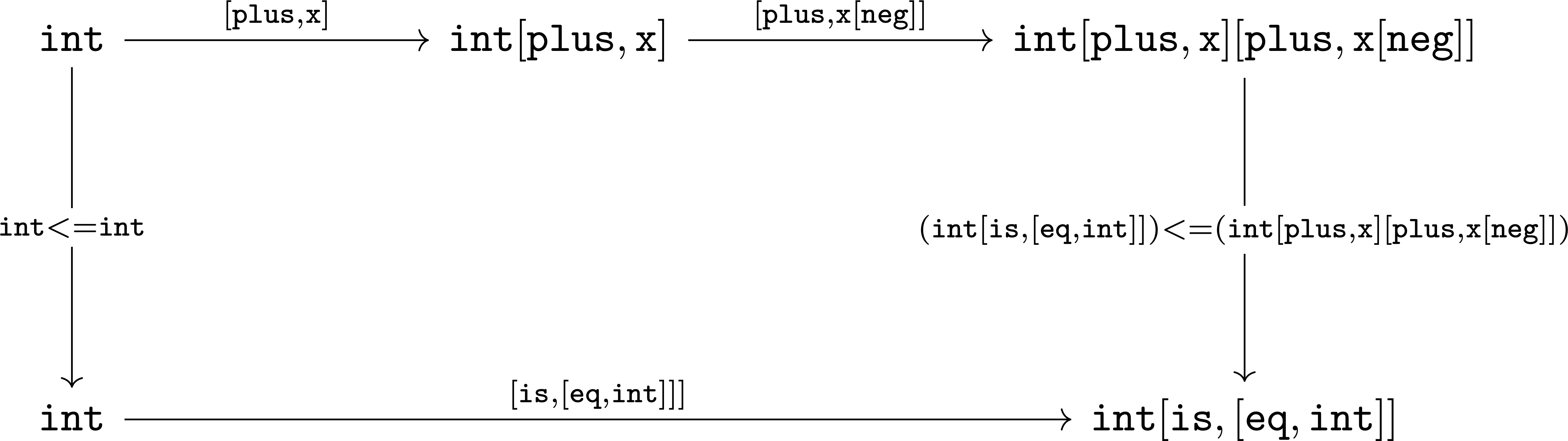
Type Patterns
| type | description | mmlang example |
|---|---|---|
A type with an unspecified domain. |
|
|
A primitive type that is a single term and coefficient. |
|
|
A composite type containing a linearly combination of terms and their coefficients. |
|
|
A subset of another type. |
|
|
A type with components of the same type. |
|
|
A type with a definition variable to the incoming |
|
|
A set of types and path equations. |
|
Refinement Types
Refinement types extend a language’s base types with predicates that further refine (constrain) the base type values. A classic example is the set of natural numbers (\$\mathbb{N}\$) as a refinement of the set of integers (\$\mathbb{Z}\$), where \$\mathbb{N} \subset \mathbb{Z}\$. In set builder notation, specifying the set of integers and a predicate to limit the set to only those integers greater than 0 is denoted
\[
\mathbb{N} = \{n \in \mathbb{Z} \;|\; n > 0\}.
\]
In mm-ADT, the above is written int[is>0] which is the sugar form of int{?}<=int[is,[gt,0]].
mmlang> :[model,mm][define,nat<=int[is>0]]
==>_[define,nat<=int[is,bool<=int[gt,0]]]
mmlang> 10 => nat
==>nat:10
mmlang> -1 => nat
language error: -1 is not a nat
mmlang> 10 => nat[plus,5]
==>nat:15
mmlang> 10 => nat[plus,5][plus,-15]
language error: 0 is not a natDependent Types
mmlang> :[model,mm][define,vec:(lst,int)<=lst-<(_,=(_)>-[count]),
                                  single<=vec:(lst,is<4).0[tail][head],
                                  single<=vec:(lst,is>3).0[head]]
==>_[define,vec<=lst[split,(lst,int<=lst[combine,(_)][merge][count])],single<=vec:(lst,_[is,_[lt,4]])[get,0,_][tail][head],single<=vec:(lst,_[is,_[gt,3]])[get,0,_][head]]
mmlang> (1;2;3)   => vec                                               (1)
==>vec:((1;2;3),1)
mmlang> (1;2;3)   => vec => single                                     (2)
==>single:1
mmlang> (1;2;3;4) => vec                                               (3)
==>vec:((1;2;3;4),1)
mmlang> (1;2;3;4) => vec => single                                     (4)
==>single:1| 1 | A ;-lst of 3 terms is morphed into a vec using the vec<=lst type. |
| 2 | The vec is morphed into a single using the first single<=vec type. |
| 3 | A ;-lst of 4 terms is morphed into a vec. |
| 4 | The vec is morphed into a single using the second single<=vec type. |
Recursive Types
A recursive type’s definition contains a reference to itself. Recursive type definitions require a base case to prevent an infinte recursion. Modern programming languages support generic collections, where a list can be defined to contain a particular type. For example, a lst containing only ints.
mmlang> :[model,mm][define,xlist<=lst[[is,[empty]]|
                                      [[is,[head][a,str]];
                                       [is,[tail][a,xlist]]]]]
==>_[define,xlist<=lst[lst{?}<=lst[is,bool<=lst[empty]]|lst{?}<=lst[lst{?}<=lst[is,bool<=lst[head][a,str]];lst{?}[is,bool{?}<=lst{?}[tail][a,xlist]]]]]
mmlang> ( ) => [a,xlist]
==>true
mmlang> ('a';'b';'c') => [a,xlist]
==>true
mmlang> ('a';'b';'c') => xlist
==>xlist:('a';'b';'c')
mmlang> (1;'a';'c') => xlist
language error: (1;'a';'c') is not a xlist
mmlang> ('a';'b';'c') => xlist[put,0,3]
language error: (3;'a';'b';'c') is not a xlist
mmlang> :[model,mm][define,ylist<=lst[[is,[empty]]|
[[is,[head][a,str]];
[is,[tail][head][a,int]];
[is,[tail][tail][a,ylist]]]]]
==>_[define,ylist<=lst[lst{?}<=lst[is,bool<=lst[empty]]|lst{?}<=lst[lst{?}<=lst[is,bool<=lst[head][a,str]];lst{?}[is,bool{?}<=lst{?}[tail][head][a,int]];lst{?}[is,bool{?}<=lst{?}[tail][tail][a,ylist]]]]]
mmlang> ( ) => [a,ylist]
==>true
mmlang> ('a';1;'b';2) => [a,ylist]
==>true
mmlang> ('a';1;'b';2) => ylist
==>ylist:('a';1;'b';2)
mmlang> (1;'a';'c') => ylist
language error: (1;'a';'c') is not a ylist
mmlang> ('a';1;'b';2) => ylist[put,0,3]
language error: (3;'a';1;'b';2) is not a ylistReference
mmlang Grammar
obj   ::= (type | value)q
value ::= vbool | vint | vreal | vstr
vbool ::= 'true' | 'false'
vint  ::= [1-9][0-9]*
vreal ::= [0-9]+'.'[0-9]*
vstr  ::= "'" [a-zA-Z]* "'"
type  ::= ctype | dtype
ctype ::= 'bool' | 'int'  | 'real' | 'str' | poly | '_'
poly  ::= lst | rec | inst
q     ::= '{' int (',' int)? '}'
dtype ::= ctype q? ('<=' ctype q?)? inst*
sep   ::= ';' | ',' | '|'
lst   ::= '(' obj (sep obj)* ')' q?
rec   ::= '(' obj '->' obj (sep obj '->' obj)* ')' q?
inst  ::= '[' op(','obj)* ']' q?
op    ::= 'a' | 'add' | 'and' | 'as' | 'combine' | 'count' | 'eq' | 'error' |
          'explain' | 'fold' | 'from' | 'get' | 'given' | 'groupCount' | 'gt' |
          'gte' | 'head' | 'id' | 'is' | 'last' | 'lt' | 'lte' | 'map' | 'merge' |
          'mult' | 'neg' | 'noop' | 'one' | 'or' | 'path' | 'plus' | 'pow' | 'put' |
          'q' | 'repeat' |'split' | 'start' | 'tail' | 'to' | 'trace' | 'type' | 'zero'
Instructions
The mm-ADT VM instruction set architecture is presented below, where the instructions are ordered by their classification and within each classification, they are ordered alphabetically.
Branch Instructions
Branch instructions enable the splitting, composing, and merging of streams. This subset of inst is a particular type of additive category called a traced monoidal category, where [repeat] provides feedback and each instruction’s poly arguments are biproducts maintaining both injective and projective morphisms. There exists a well-established graphical language for such monoidal categories that has been adopted in mmlang sugar syntax (or as best as can be reasonably captured using ASCII characters).
| name | string diagram | sugar | mmlang example |
|---|---|---|---|
initial |
|
|
|
split |
|
|
|
merge |
|
|
|
repeat |
|
|
|
terminal |
|
|
|


| inst | description | example |
|---|---|---|
|
Juxtapose start across |
|
|
Pairwise juxtapose the terms of two |
|
|
Detach from the |
|
|
Aggregate the terms of the start |
|
|
Apply the first \[ x(a^n) = x \prod^{i \leq n}_{i=0} a \] |
|
|
Juxtapose start across |
|
|
Replace the |
|